Bayesian Filter
Over the last 6 months on and off, I’ve built myself a bayesian spam filter. In this article I’ll give an overview of the thing, the theory behind it and the experiences I’ve had and the things I’ve learned while building it.
Intro
Bayesian spam filters classify email messages into basically two categories:
- “Spam”, i.e. unwanted messages such as advertisement
- “Ham”, i.e. wanted messages such as corrospondence from friends
There are gray areas between these two when a filter does not know how to classify a message.
Note: this is a slightly expanded, translated version of a talk I held in April 2021 on C3PB’s Mumble server.
All errors in this text are mine and mine alone. I’m not a mathematician by training or trade so a lot of the theory explained below may be abridged to the point of uselessness, explained in a way that noone but myself understands or plain wrong. If you notice anything, please be so kind and tell me about it.
Why?
Bogofilter, which is what I used before, is a bit opaque, at least to me, and it had a few performance issues in my setup, especially when bulk training messages.
Also, I wanted to learn what makes Spam/Ham classification work, and to see whether I have the skills (or could learn them) needed to build a resonably good mail filter.
Goal(s)
I built my filter with the following goals in mind:
- I can live with false negatives: Spam that is not recognized as such
- I want to keep the number of false positives, i.e. messages classified as Spam even though they were Ham, as low as possible
- (reasonably) fast training time:
- Train my personal archive of OpenBSD’s “Misc” mailing list (roughly 70k messages) as “Ham” in less than 5 minutes.
The last part is especially important to me, though it may not be a good idea to bulk train that many messages. Bogofilter took upwards of 45 minutes to perform that training.
Basics
Conditional Probability/Bayes
We count how often we see a word (in this context, “word” refers to “a sequence of interesting bytes”) in the context “Spam” or “Not Spam” (i.e. Ham).
These counts lead us to the following (estimated) probabilities:
- $P(W|S)$
- $P(W|H)$
TODO : Expand: how are these calculated?
$P(W|S)$ meaning “The probability of seeing word $W$ in the context of a Spam message”.
In the talk, I claimed that $P(W|H) = 1 - P(W|S)$, but that is not quite correct. The probability of a word being seen in the context of a Spam message is indepentend of the probability of the word being seen in the context of a Ham message, since these form two completely separate “populations” of messages: a message is either Ham or Spam, but never both.
From these probabilities, we can derive the following probabilities that form the core of the classification engine:
- $P(S|W)$: Probability of a message being Spam, given that we’ve seen the word $W$
- $P(S|M)$: Probability of a message being Spam, given all the words in the message $M = W_1 W_2 \ldots W_n$
As mentioned above, I use the term “word” in a slightly more generic term than is common: A word is a sequence of “interesting” characters, for some measure of “interesting”.
Single words
To calculate $P(S|W)$, we use the following equation:
$$ P(S|W) = \frac{P(W|S)}{P(W|S) + P(W|H)} $$
We know all elements of this equation:
- $P(W|S)$: how often have we seen $W$ in the context of a Spam message?
- $P(W|H)$: how often have we seen $W$ in the context of a Ham message?
“How often” is relative: if we’ve seen $W$ a total of 236 times, 46 of which were in the context of a Spam message, the scores come out to:
$$ \begin{align} P(W|S) &= \frac{46}{236} \approx 0.1949 \\ P(W|H) &= \frac{236 - 46}{236} = \frac{190}{236} \approx 0.805 \\ P(S|W) &= \frac{P(W|S)}{P(W|S) + P(W|H)} = \frac{\frac{46}{236}}{\frac{46}{236} + \frac{190}{236}} \end{align} $$
TODO: Verify the math here. This looks wrong: Why is the numerator always 1? Is that correct?
Complete messages
To estimate the probability that a given message $M = W_1 W_2 \ldots W_n$ is Spam, we combine the probabilities that each of its constituent words is Spam:
$$ \begin{align} p_n &= P(S|W_n) \\ P(S|M) &= \frac{p_1 \cdot p_2 \cdot \ldots \cdot p_n}{p_1 \cdot p_2 \cdot \ldots \cdot p_n + (1-p_1) \cdot (1-p_2) \cdot \ldots \cdot (1-p_n)} \end{align} $$
The form of this equation somewhat mirrors how we calculate the Spam probability for a single word.
Math tricks #1: Logarithms
To prevent over/underflow when multiplying potentially thousands of per-word probabilities, we use logarithms:
$$ \begin{align} \log \frac{x}{y} &= \log x - \log y \\ \log xy &= \log x + \log y \end{align} $$
Instead of computing $p = \frac{p_0 \cdot p_1 \cdot \ldots \cdot p_n}{p_0 \cdot p_1 \cdot \ldots \cdot p_n + (1-p_0) \cdot (1-p_1) \cdot \ldots \cdot (1-p_n)}$, we compute $p$ like this:
$$ \begin{align} \eta &= \sum_{x=0} \log(1-p_x) - \log p_x \\ p &= \frac{1}{1+e^\eta} \end{align} $$
This prevents over and underflow during multiplication, because $P(x)$ is in the interval $[0, 1]$ (since it is a probability). This keeps $\log(P(x))$ in a range that’s relatively easy to manage:
- $\log 0.05 \approx -2.9957$
- $\log 0.95 \approx -0.0513$
Since the proof is in the pudding, this is how we derive the sum:
\begin{align} p &= \frac{p_0 \cdot p_1 \cdot \ldots \cdot p_n}{p_0 \cdot p_1 \cdot \ldots \cdot p_n + (1-p_0) \cdot (1-p_1) \cdot \ldots \cdot (1-p_n)} \\ \Rightarrow \frac{1}{p} &= \frac{(1-p_0) \cdot (1-p_1) \cdot \ldots \cdot (1-p_n)}{p_0 \cdot p_1 \cdot \ldots \cdot p_n} + \frac{p_0 \cdot p_1 \cdot \ldots \cdot p_n}{p_0 \cdot p_1 \cdot \ldots \cdot p_n} \\ \Rightarrow \frac{1}{p} - 1 &= \frac{(1-p_0) \cdot (1-p_1) \cdot \ldots \cdot (1-p_n)}{p_0 \cdot p_1 \cdot \ldots \cdot p_n} \\ &= \frac{1-p_0}{p_0} \cdot \frac{1-p_1}{p_1} \cdot \ldots \cdot \frac{1-p_n}{p_n} \\ \Rightarrow \log \left( \frac{1}{p}-1 \right) &= \sum_{x=0} \log (1-p_x) - \log p_x = \eta \\ \Rightarrow \frac{1}{p} - 1 &= e^\eta \\ \Rightarrow p &= \frac{1}{1 + e^\eta} & \Box \end{align}
Math tricks #2: Sigmoid function
Since division by 0 for $P(x) \in \lbrace 0, 1 \rbrace$ isn’t defined, we need to special-case it. The easiest way to do that is to make sure that $P(x)$ is never equal to $0$ or $1$. My approach for that is to use a tuned sigmoid funtion that is strictly greater than 0 and less than 1 in the interval $[0, 1]$:
$$ \sigma (x) = \frac{1}{1 + e^{-k (x-m)}} $$
for $k = 5$ and $m = 0.5$. This ensures that $0 < \sigma (P(x)) < 1$.
Note that I could’ve used something like this:
$$ \sigma (x) = \min \left( \max \left( x, 0.1 \right), 0.99 \right) $$
to ensure roughly the same constraints, but a real sigmoid seemed nicer to me since it’s a smooth curve. Not that that would be important here, it’s just nice to look at.
Counting Bloom filters
For counting and storing relative frequencies of words, I use a Counting Bloom Filter. My reasoning for that is that the list of words that the filter might encounter is potentially endless, which leads to unpredictable storage demands and lookup times.
A counting bloom filter has constant space usage and constant lookup/update time, at the cost of providing only an estimation of the actual count. In this case that is okay though since the data that’s being fed into the filter is of stochastic nature anyway.
Basics: Bloom Filters
A bloom filter (of the non-counting variant) is a collection of $k$ hash functions and a set of bit fields $F_1 \ldots F_k$ (i.e. one for each hash function), of size $n$.
To store a word $w$ in the filter, we need to perform the following steps:
- Compute $k$ hashes for $w$, one for each hash function: $\rightarrow h = \left[ h_1, h_2, …, h_k \right] \mod n$
- In each bit field $F_x$, set the bit indicated by hash $h_x$: $F_x[h_x] \leftarrow 1$
To answer the question “Has $w$ been added to the filter?” we answer the question “Is every bit in $h$ set in the appropriate bit field?”.
Since hashes can have collisions, the answer to this question is either:
- “$w$ may habe been added to the filter” (the bits might have been set through collisions of unrelated words)
- or “$w$ has definitely never been added to the filter”
$$ w \in F \Leftrightarrow \forall x\in \left[0, \ldots , k \right]: F_x[h_x(w)] = 1 $$
Extension to counting bloom filters
Counting bloom filteres extend classical bloom filters by storing an integer instead of a single bit. Adding a word to the filter then means increasing the counters instead of setting bits, and the counter value for a word is the minimum counter in each of the fields of the filter.
This sort of filter can overestimate how often a word has been seen by a filter (since the counters may be modified through unrelated words), but it will never under-estimate the count.
This is an example of a filter with $k = 4$ and $n = 10$ into which two words $w_1$ and $w_2$ are added:
$$h(w_1) = \left[ 5, 7, 3, 9 \right] , h(w_2) = \left[ 4, 9, 3, 1 \right]$$
This illustrates a bit how the counters are updated:
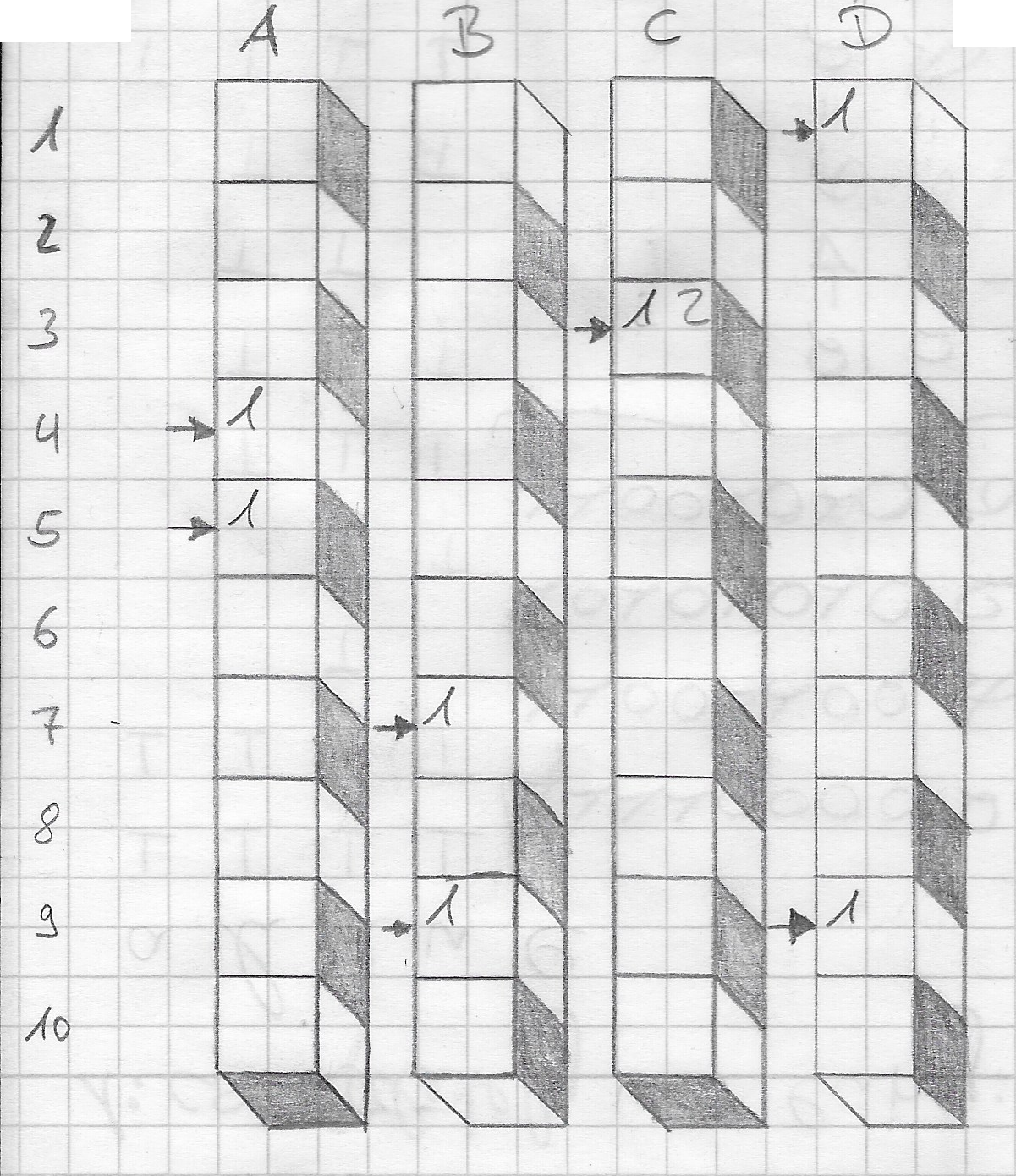
A counting bloom filter
In the example, there are four hash functions ($A$, $B$, $C$, $D$). Words with the following hashes are inserted:
- $h(w_1) = \left[ 4, 7, 3, 1 \right]$
- $h(w_2) = \left[ 5, 9, 3, 9 \right]$
There is a collision at $C_3$, which means that instead of just flipping a bit, we increase the value stored there. To get an estimate of how often $w_1$ was stored, we count the minimum of all hash fields and see that it was stored once. The same goes for $w_2$.
Usage in my mail filter
My filter uses three counting bloom filters that each store uint32 counter values:
- One for storing the total number of times that a word has been seen
- One for storing how often a word has been seen in a spam message
- One for storing how often a word has been seen in a ham message
The filters are persisted once a minute and are locked by a single sync.RWLock, which allows concurrent read of the filter but serializes write updates. This reflects the fact that the filter is used more often in a reading more (when classifying new mail) than in training mode.
The filters use FNV-1 as their hash function, which has the disadvantage that it does not have an avalanche effect. Words that are “similar” will have similar hash values, but it’s reasonably fast, since it’s only a single multiplication and XOR per hashed byte.
Advantages and disadvantages
Using a set of counting bloom filters to store word frequencies has the following advantages:
- Lookup and Insert in $O(|w|)$, which is almost constant time (since words are small)
- Constant space usage:
- ~64MB per bloom filter for $n = 1 000 000$ and $k = 16$
It also has these disadvantages:
- All filters have to be in RAM at all times
- Cache locality is very bad
- there is only one direction for mapping
- I can’t tell you what the word with the highest Spam score is, but if you tell me a word, I can tell you its score
- The collision probability increases with usage, which makes the counts imprecise. Since this affects both total and specific counts (ham/spam), the effects of this stay manageable.
TODO
- Some calculations re: performance, probability of collisions, density
My design
Plan
- Collect word frequencies (= training)
- To evaluate a message as Ham or Spam:
- Map each word to its Spam frequency
- Compute the probability that the message is Spam using Bayes rule
- Threshold:
- $p \le 0.3$ → “ham”,
- $p \ge 0.7$ → “spam”,
- everything in between: “unsure”
Actual outcome
- Go, 1589 LOC (~ 736 LOC Tests/Benchmarks)
- Almost no usage of packages outside of Go’s standard library besides
github.com/pkg/errors
- Almost no usage of packages outside of Go’s standard library besides
- REST-API with POST-Requests:
/train?as={ham,spam}&factor=23for training/classify?mode={plain,email}&verbose={true,false}for classification
- Frequencies are stored in a set of counting bloom filters
- Messages are segmented with a sliding window ($n = 6$)
To integrate it into my “read and write mail” workflow:
- the service is running permanently as part of my user session (
systemduser sessions rule, by the way) - I use
maildropas the local MDA, and it’s configured toxfiltermessages through the mail filter - Keybindings in
neomuttfor training individual (sets of) messages and to check classification
Ideas that didn’t work out
These are ideas that I’ve tried out and abandoned, either because they’re completely wrong or because implementing them made the code more complex than I wanted it for too little gain:
- Normalizing message content, i.e. stripping out/replacing punctuation or digits does not influence results nearly as much as expected
- exponential decay of $\eta$
- Complete nonsense because it means that the end of messages completely drowns out things like the headers in the beginning.
- SQLite, BoltDB, selfmade K-V Store with WAL as Data Store
- Counting Bloom Filter beats them all in speed and storage space requirements, for very little downsides
- … and is a lot easier to read, code-wise
- Clever Dirty-Maps for partially writing updated bloom filters, such as
- VEB-Trees
map[int]struct{}with lazy Extent Coalescion- … It turns out that just writing out the complete filter data every once in a while (only if the filter has been updated of course) is just as fast and easier to understand.
Lessons learned and things that helped a lot during building the service
- Profiling, especially the ability to run a profiler on a “production” instance of the service (through
go tool pprofandnet/http/pprof) - Verbose debugging to answer the question “Why the hell was this message evaluated as Spam?”
- In the beginning, I ran my filter after
bogofilter. This caused my filter to start training on Bogofilter’s annotation headers. If bogofilter said a message is ham, my filter said so as well, but only because there wereX-Bogosityheaders in the message to that effect, not because of the message itself.
Benchmarks and tests
Make benchmarks often, and design them so that they are part of your test suite (if that’s possible). Build the test suite while you’re doing development, not “after the features are done”. Tests built after the fact are not as good as tests that evolve together with the code that they test.
Test driven development also allows you to focus on the pieces that you’re currently working on, even if the rest of the project is still a “construction site”.
Try to collect application specific metrics in your benchmarks, not just “time per operation”. These could be things like:
- Hit rate in caches
- Collision rate in bloom filters
- Storage overhead
- Number of network packets transmitted
- Precision and specificity of a classification system
It’s also important to at least think about how to justify the performance of things that are “fast enough”. Some times, things that you consider “pretty fast I guess” can be improved by orders of magnitude if you know where to look.
When deciding which data to use for benchmarks, try to approximate real world usages. Algorithms that perform just right for $n=10\text{k}$ might:
- be too slow/use too much space for $n=100 \text{ million}$
- be too complex for $n=100$
As a case in point, while developing the frequency store based on counting bloom filters, I used real frequency data from previous implementations of the filter that used BoltDB for storage. This data was representative of the kind of data that the bloom filter would have to store, since it had been collected over a few weeks of usage.
A single instance of a benchmark does not say much when it stands alone: does “100 operations/second” mean it’s fast? Or is that slow? Is it faster/slower than before?
You should collect benchmark results from different iterations of your code so that you can see where you’re heading, and see when you start going into the wrong direction. This is especially important when you embark on a “let’s make this faster” journey. The workflow should be:
- Write a benchmark for the area in question/make sure existing benchmarks work
- Check that the data the benchmark uses at least approximate the environment that your code will later run in
- Run a few instances of the benchmark and save their results
- Make your changes
- Run the same benchmark that you used to evaluate your old code again. No changing parameters!
After that, you can compare the results and actually show that your changes made everything faster (or maybe that they made things acceptably slower).
Benchmarks can be compared with benchstat:
$ benchstat old.txt new.txt
name        old time/op  new time/op  delta
GobEncode   13.6ms ± 1%  11.8ms ± 1%  -13.31% (p=0.016 n=4+5)
JSONEncode  32.1ms ± 1%  31.8ms ± 1%     ~    (p=0.286 n=4+5)
Have a goal in sight
- here: a concrete maximum duration for training a specific data set
- also: build a mail filter that does exactly one thing: classify RFC822 messages into either “ham”, “spam” or “unsure”
- … and that is easy to integrate into my existing mail reading pipeline.
Be flexible
Try not to focus your design on the aspects of a specific data store, play around with different algorithms and data structures, and be ready to make tradeoffs:
- precise frequencies vs. quick updates/constant storage
- long lived server processes vs. oneshots
Things that may or may not come in the future
- More labels than Ham/Spam using a Maximum-Likelihood Estimator:
ccc,bills,bank
- Multi-Tenancy with interesting privacy implications:
- Who is allowed to train the filter?
- How strongly does training done by user X influence classification done by user Y?
- Leaks: “Viagra isn’t recognized as Spam anymore? Someone must have trained it as ham!”
- Make message parsing smarter
- Skip attachments such as PGP keys or images
- Put more focus on headers
- Dropout repeated or rarely used words